Customizing colors in R
Colors can be defined in R in at least three ways: by number, by name and by RGB designation. There are other color palette packages such as RColorBrewer that provide additional control over color schemes.
Color numbers
There are 8 color numbers to choose from, for example:

Color names
R offers a big list of color names–too big to list on this page. The names can be accessed via the colors() function.
colors()In the following example, we display a subset of these colors.

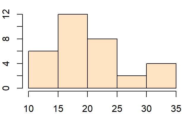
So if you wan to use a bisque color in your histogram, type:
hist(mtcars$mpg, col = "bisque", main = NULL, xlab = NULL, ylab = NULL)
RGB designation
Colors can also be defined by the computer display’s primary colors; red, green and blue (RGB for short). One can use the rgb() function to define the levels of each primary color from a scale of 0 to 1 with one being the color’s maximum intensity. For example, if you want to generate a pure blue color, type:
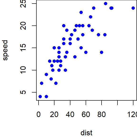
rgb(0,0,1)[1] "#0000FF"The function returns a hexadecimal value, #0000FF, which R can convert to a color. For example to plot blue points, type:
plot( speed ~ dist, cars, pch=16, col=rgb(0,0,1))
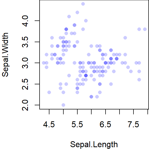
A fourth parameter can be passed to rgb(): the opaqueness value alpha. This is useful when many overlapping points are displayed on a plot. alpha is defined in an interval from 0 to 1 with 1 being completely opaque and 0 being completely transparent. In the following example, we apply a blue color to the dots and assign them a 80% transparency (opaqueness = 0.2):
plot( Sepal.Width ~ Sepal.Length, iris , pch=16, col=rgb(0,0,1, 0.2))
